네 번째 프로젝트
프로젝트를 하면서 느낀 보완사항은 :
-데이터의 길이가 너무 짧으면 단어를 추출하는데 한계가 있고, 과적합이 발생한다.
-유의미한 단어가 존재해야 정확도가 더 개선된다. 모델을 계속 만져봐도 정확도는 크게 개선되지 않는다.
-각 사이트마다 카테고리 분류가 다르게 되어있어서 소비자가 불편할 수도 있을 것이다.
|
1
2
3
4
5
6
7
8
9
10
11
12
13
14
15
16
17
18
19
20
21
22
23
24
25
26
27
28
29
30
31
32
33
34
35
36
37
38
39
|
# 모듈 임포트
import pandas as pd
import numpy as np
from tensorflow.keras.utils import to_categorical
from sklearn.model_selection import train_test_split
from sklearn.preprocessing import LabelEncoder
from tensorflow.keras.preprocessing.text import *
from tensorflow.keras.preprocessing.sequence import pad_sequences
import pickle # pickle을 이용하면 int 값을 그대로 저장하고 그대로 불러옴
from konlpy.tag import Okt # 형태소 분리기 임포트
pd.set_option('display.unicode.east_asian_width',True)
df = pd.read_csv('/content/10x10(kor2).csv', index_col=0)
print(df.head())
print(df.info())
# 중복 행 확인
col_dup = df['title'].duplicated()
print(col_dup)
sum_dup = df.title.duplicated().sum()
print(sum_dup)
# title 컬럼 기준으로 중복 제거 (row 통째로 제거)
df = df.drop_duplicates(subset=['title'])
sum_dup = df.title.duplicated().sum()
print(sum_dup)
# 인덱스 새로 고침
df.reset_index(drop=True, # False로 줄 시 기존 인덱스를 colum으로 올림
inplace=True)
print(df.head())
print(df.tail())
|
cs |
이 과정만 잘 따라와도 누구나 쉽게 카테고리 분류가 가능하다.
|
1
2
3
4
5
6
7
8
9
10
11
12
13
14
15
16
17
18
19
20
21
22
23
24
25
26
|
# 데이터 나누기
X = df['title']
Y = df['category']
# 원핫인코딩 위해 라벨로 변경
encoder = LabelEncoder()
labeled_Y = encoder.fit_transform(Y)
label = encoder.classes_
# 지정한 라벨 저장
# 이미 학습한 라벨들을 이용해야 학습된 결과들과 똑같이 도출
with open('/content/10x10_category_encoder.pickle', 'wb') as f:
pickle.dump(encoder, f)
# 원핫인코딩 => 정답데이터 원핫인코딩(희소벡터처리)
onehot_Y = to_categorical(labeled_Y)
# 첫번째 데이터 형태소로 분리
okt = Okt()
okt_X = okt.morphs(X[0])
# 모든 row를 형태소로 분리
for i in range(len(X)):
X[i] = okt.morphs(X[i])
|
cs |
추후에 데이터들을 불러서 모델 성능이 얼마나 좋은지 평가를 하기 위해서 라벨들을 통일시켜야 한다.
|
1
2
3
4
5
6
7
8
9
10
11
12
13
14
15
16
17
18
|
# stopwords 불러오기
stopwords = pd.read_csv('/content/stopwords2.csv')
# stopwords에 있는 단어를 제거하고 리스트에 담기
words = [] # 빈 리스트 생성
for word in okt_X:
if word not in list(stopwords['stopword']):
words.append(word)
#한 행씩 모든 데이터 처리
for i in range(len(X)): # X=df['title']
result = []
for j in range(len(X[i])):
if len(X[i][j]) > 1:
if X[i][j] not in list(stopwords['stopword']):
result.append(X[i][j])
X[i] = ' '.join(result)
|
cs |
불용어 제거 단계
|
1
2
3
4
5
6
7
8
9
10
11
12
13
14
15
16
17
18
19
20
21
22
23
24
25
26
27
28
29
30
31
32
|
#단어를 컴퓨터에서 인식시키기 위해 각 단어마다 숫자(라벨링) 부여 => 토큰화
# 수치적인 의미는 없음
token = Tokenizer()
token.fit_on_texts(X)
tokened_X = token.texts_to_sequences(X)
print(tokened_X[0])
#읽고 쓰는 과정에서 데이터의 자료형을 따로 인코딩할 필요 없이 그대로 저장
import pickle
with open('/content/10x10_token3.pickle', 'wb') as f:
pickle.dump(token, f)
wordsize = len(token.word_index) + 1
max = 0
for i in range(len(tokened_X)):
if max < len(tokened_X[i]):
max = len(tokened_X[i])
#LSTM모델 사용을 위해 데이터 크기가 다른 것들을 0을 채워넣어 max사이즈로 통일시킴
X_pad = pad_sequences(tokened_X, max)
X_train, X_test, Y_train, Y_test = train_test_split(
X_pad, onehot_Y, test_size=0.1)
print(X_train.shape)
print(X_test.shape)
print(Y_train.shape)
print(Y_test.shape)
xy = X_train, X_test, Y_train, Y_test
np.save('/content/10x10_data_max_{}_size_{}_2'.format(max, wordsize), xy)
|
cs |
언어를 컴퓨터가 이해하기 위해서 토크나이징 과정을 거친다.
|
1
2
3
4
5
6
7
8
9
10
11
12
13
14
15
16
17
18
19
20
21
22
23
24
25
26
27
28
29
30
31
32
33
34
35
36
37
38
39
40
|
import pandas as pd
import numpy as np
import matplotlib.pyplot as plt
from tensorflow.keras.models import Sequential
from tensorflow.keras.layers import *
from keras.callbacks import EarlyStopping
X_train, X_test, Y_train, Y_test = np.load(
'/content/datasets/10x10_data_max_13_size_20320_2.npy',
allow_pickle=True)
#max: 한 행의(리스트 글자의) 최대 길이
#size: 차원 수
##모델 생성
model = Sequential()
#X_pad로 사이즈 통일시킨 데이터를 embedding layer가 원핫인코딩+벡터라이징 처리해줌
#벡터라이징: 각 인덱스별 의미부여를 벡터공간이라는 개념을 도입해 처리
model.add(Embedding(20320, 300, input_length=13))
#차원수 20320를 차원수 300으로 낮추고 input_length는 max최대값인 13으로 입력
model.add(Conv1D(512, kernel_size=5,
padding='same', activation='relu'))#1차원 컨볼루션=> conv1d, 2차원 컨볼루션=>conv2d
model.add(MaxPool1D(pool_size=1))
#conv다음에는 maxpool함께 감
model.add(LSTM(128, activation='tanh',
return_sequences=True))
model.add(Dropout(0.2))
model.add(LSTM(64, activation='tanh',
return_sequences=True))
model.add(Dropout(0.1))
model.add(Flatten())
model.add(Dense(128, activation='relu'))
model.add(Dense(10, activation='softmax'))#y값개수: 10(카테고리개수)
early_stopping = EarlyStopping(monitor='val_accuracy', patience=3)
# 5 에포크 동안 해당 값이 좋아지지 않으면 학습을 중단.
print(model.summary())
|
cs |
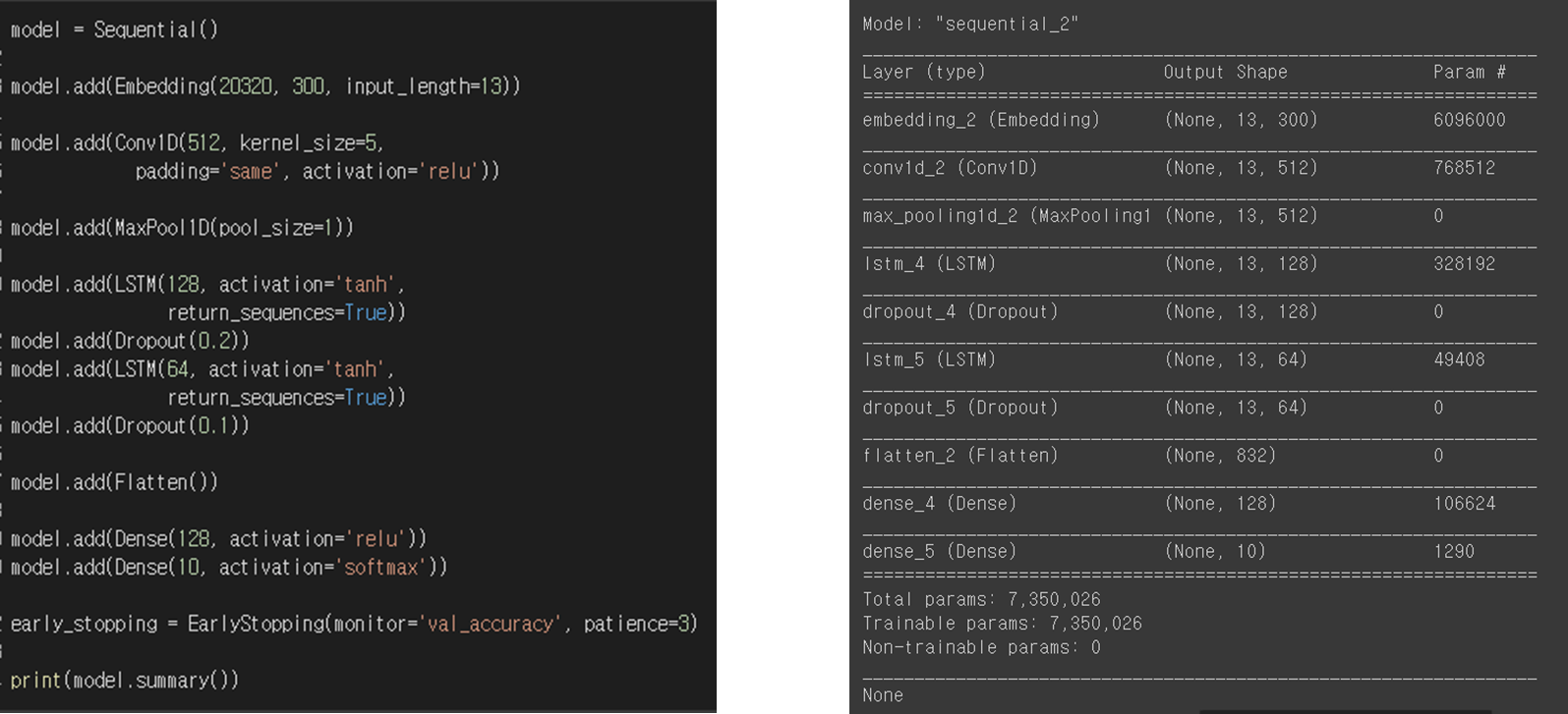
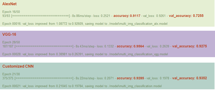
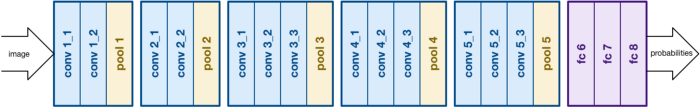
모델 구조
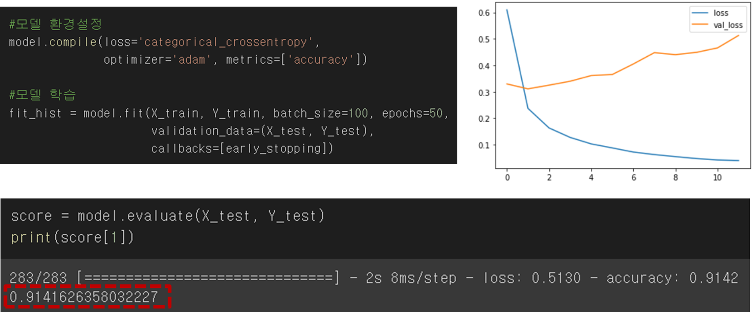
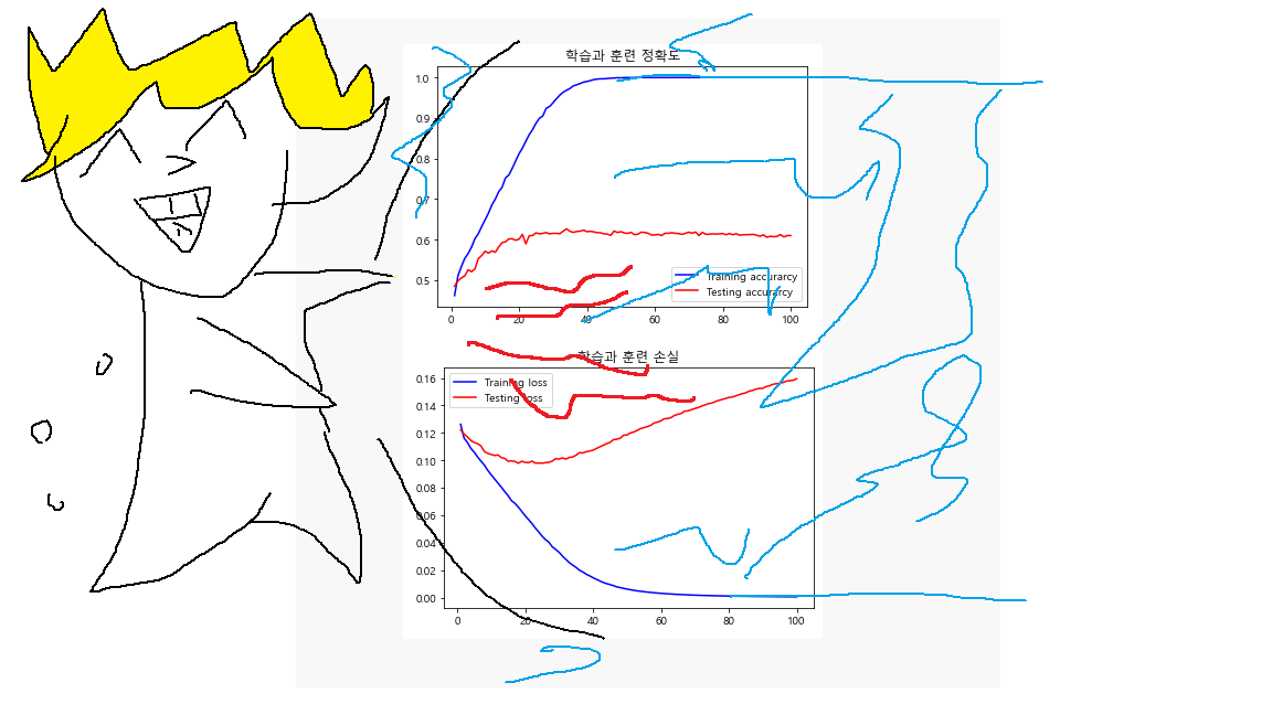
모델 정확도는 높게 나오지만 지속적으로 val_loss 값이 증가하는 것으로 보아, 약간의 과적합이 발생함을 확인했다.
제목 자체가 길지 않기 때문에 okt로 형태소 분석을 끝내고, stopwords로 불용어를 제거, 기타 전처리 과정을 끝냈을 때, 제목 최대 길이가 13밖에 나오지 않아서 그렇지 않을까 하는 추측을 해본다.
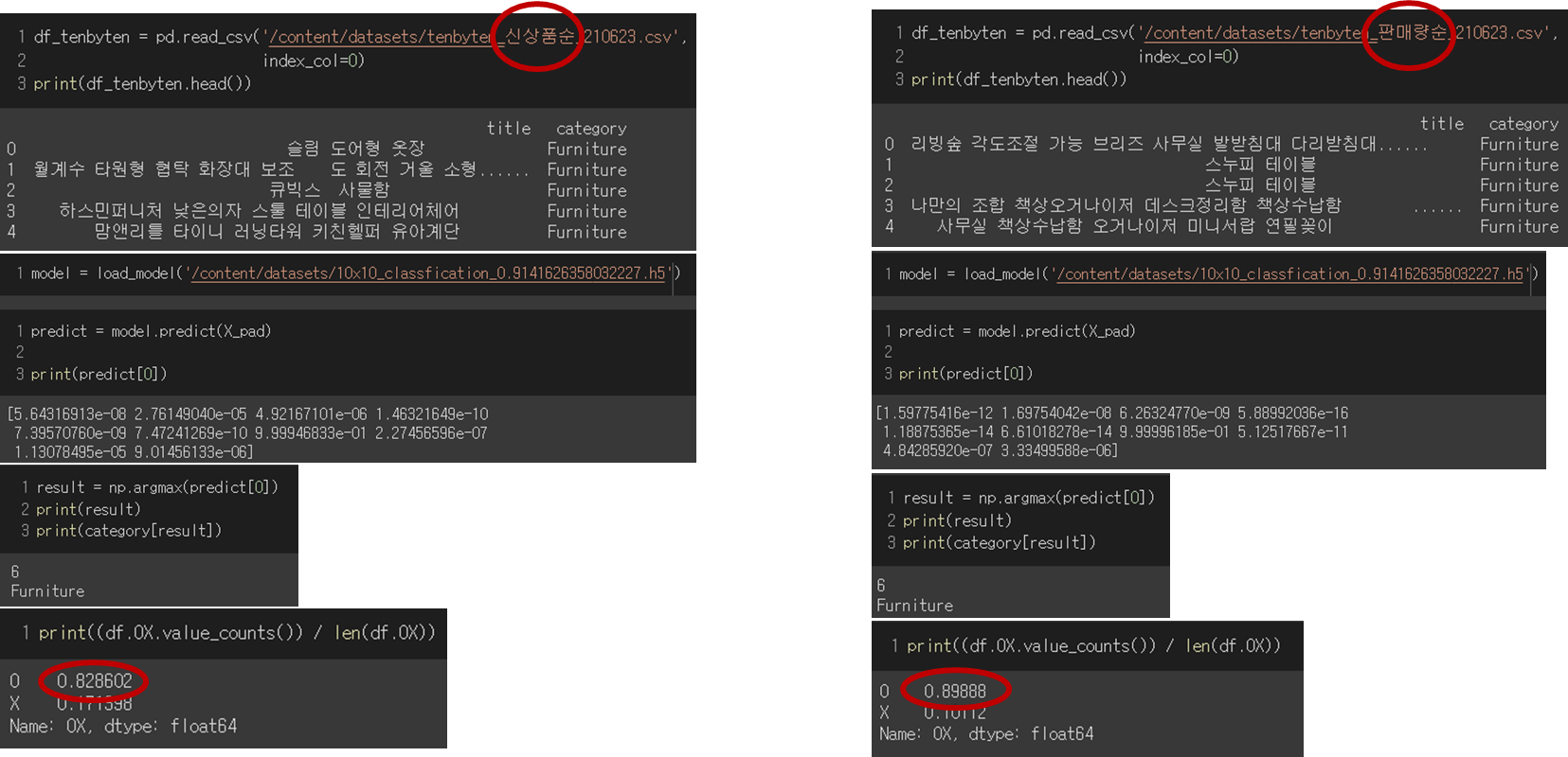
학습한 모델을 가지고 신상품순, 판매량순으로 새로 데이터를 크롤링해서 성능을 평가해보았다. 지속적으로 학습을 시키고, 더 많은 데이터를 학습시켰다면 신상품이 들어온다고 해도 정확도가 많이 떨어지지 않을 것으로 보인다.

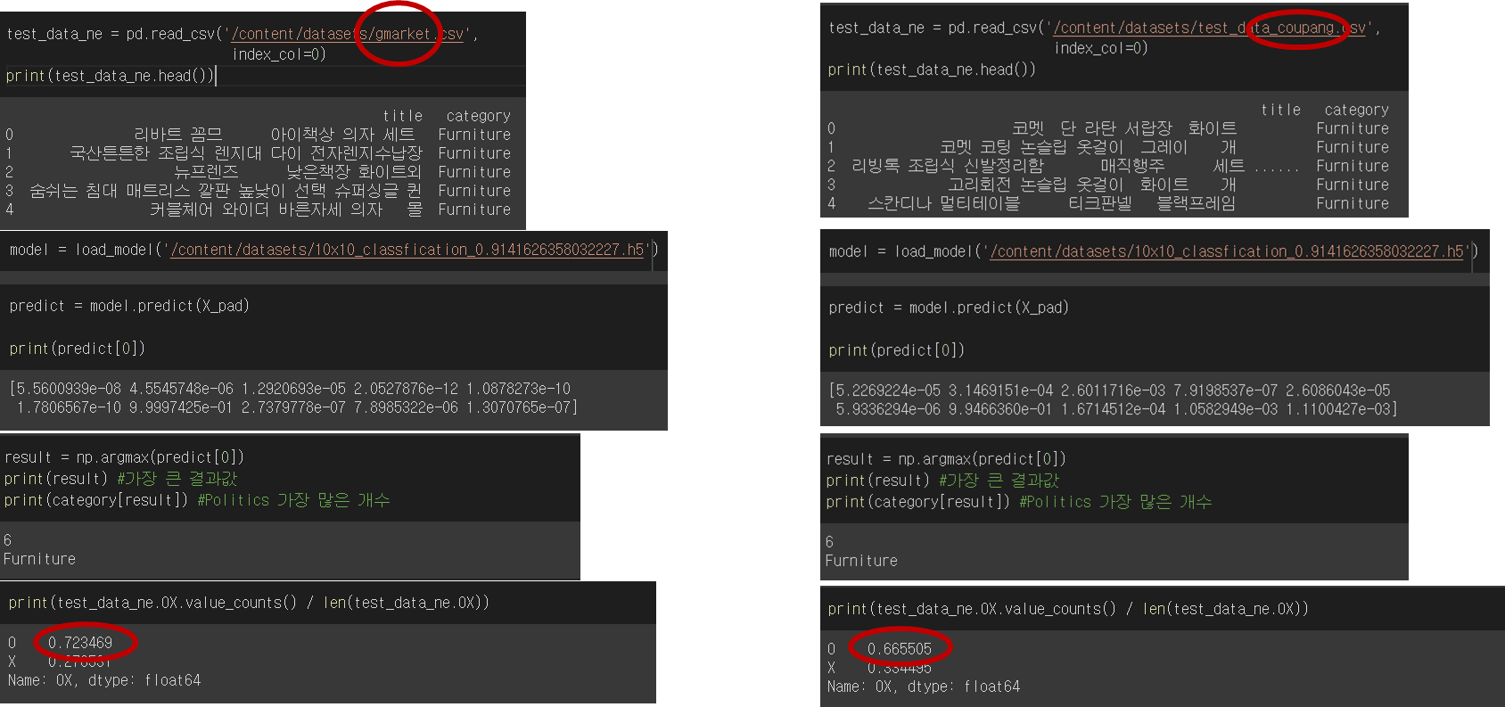
10x10으로 학습시킨 모델을 쿠팡, 지마켓에 적용하려고 하니까 성능이 확실히 떨어지는 것을 확인할 수 있다. 제목도 각 사이트마다 짓는 방법도 다를 것이며, 같은 제품이라도 다른 카테고리에 있음을 확인했다.
예를 들어, 비타민C 고려은단은 당연히 건강식에 있을거라고 생각했는데... 쿠팡에서 아이 유아쪽 카테고리에 있었다.
'도전하자. 프로젝트' 카테고리의 다른 글
| 5-2 파이썬 팀프로젝트 추천시스템 (자연어 NLP / TF-IDF, Word2Vec) (0) | 2021.08.13 |
|---|---|
| 5-1 파이썬 팀프로젝트 - 추천 시스템과 편향 방지 (유튜브의 알고리즘?) (0) | 2021.08.12 |
| 4-2 파이썬 팀프로젝트 CNN 카테고리 분류 - 데이터 크롤링 및 전처리 (0) | 2021.08.10 |
| 4-1 파이썬 팀프로젝트 CNN 상품 카테고리 분류 intro (셀리니움 vs BS4) (0) | 2021.08.10 |
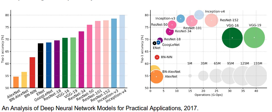
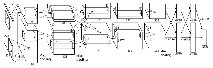
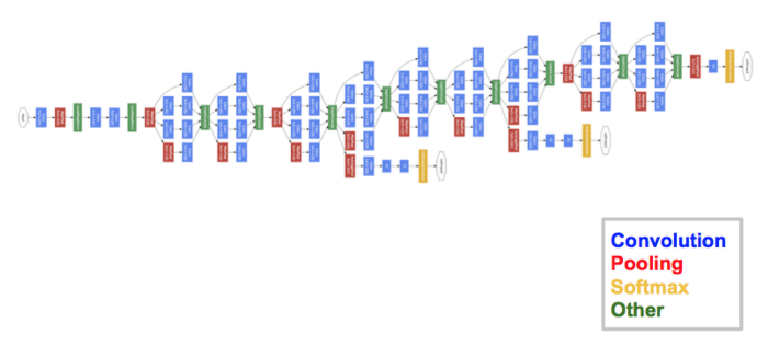
| 3-4 파이썬 팀프로젝트 - CNN, AlexNet, VGG-16 모델 평가 (0) | 2021.08.09 |