세 번째 프로젝트 순서

프로젝트 발표 준비 전 모델 평가 및 성능 테스트? 단계
참고로 그린라이트로 정하게 된 배경에는.. 예전에 마녀사냥에서 자주 사용했던 그린라이트, 불빛이 들어온다는 느낌에서 약간의 언어유희를 사용했다. 식물이 아픈지 안 아픈지 제대로 정의해준다(right)와 밝혀준다(light)의 조합이랄까..
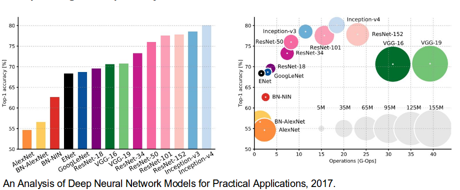
이미지 인식 모델에서 자주 사용 되는 모델 AlexNet, VGG-16, GoogleNet(2012~2014), ResNet, InceptionV3 (2014 이후) 매년 ImageNet Large Scale Visual Recognition Challenge( ILSVRV ) 대회에서 성능 비교를 한다. 요즘은 점차 정확도에 차이가 줄어서 0.01% 차이로도 순위가 갈린다고 수업시간에 들었다.
AlexNet
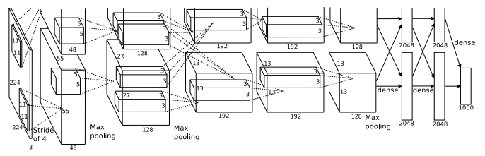
2012년 AlexNet 은 이전의 모든 경쟁자를 압도할 정도로, 상위 5개 오류를 26%에서 15.3%로 줄였다고 한다. 총 8개의 layer로 구성 됐고, 5개는 convolutional layer로 구성이 됐다. 11x11, 5x5, 3x3, 컨볼루션, 최대 풀링, 드롭아웃, 데이터 증대, ReLU 활성화 등으로 구성이 됐다.
입력 크기 256x256x3
|
1
2
3
4
5
6
7
8
9
10
11
12
13
14
15
16
17
18
19
20
21
22
23
24
25
26
27
28
29
|
def Alexnet_model():
inputs = Input(shape=(64, 64, 3))
conv1 = Conv2D(filters=48, kernel_size=(10, 10), strides=1, padding="valid", activation='relu')(inputs)
pool1 = MaxPooling2D(pool_size=(3, 3), strides=2, padding="valid")(conv1)
nor1 = tf.nn.local_response_normalization(pool1, depth_radius=4, bias=1.0, alpha=0.001/9.0, beta=0.75)
conv2 = Conv2D(filters=128, kernel_size=(3, 3), strides=1, padding="same", groups=2, activation='relu')(nor1)
pool2 = MaxPooling2D(pool_size=(3, 3), strides=2, padding="valid")(conv2)
nor2 = tf.nn.local_response_normalization(pool2, depth_radius=4, bias=1.0, alpha=0.001 / 9.0, beta=0.75)
conv3 = Conv2D(filters=192, kernel_size=(3, 3), strides=1, padding="same", activation='relu')(nor2)
conv4 = Conv2D(filters=192, kernel_size=(3, 3), strides=1, padding="same", activation='relu')(conv3)
conv5 = Conv2D(filters=128, kernel_size=(3, 3), strides=1, padding="same", activation='relu')(conv4)
pool3 = MaxPooling2D(pool_size=(3, 3), strides=2, padding="valid")(conv5)
drop1 = Dropout(0.5)(pool3)
nor3 = tf.nn.local_response_normalization(drop1, depth_radius=4, bias=1.0, alpha=0.001 / 9.0, beta=0.75)
flat = Flatten()(nor3)
dense1 = Dense(units=2048, activation='relu')(flat)
dense2 = Dense(units=1024, activation='relu')(dense1)
logits = Dense(units=20, activation='softmax')(dense2)
return Model(inputs=inputs, outputs=logits)
model=Alexnet_model()
model.summary()
model.compile(loss='binary_crossentropy', optimizer=otm, metrics=["accuracy"])
|
cs |
GoogleNet
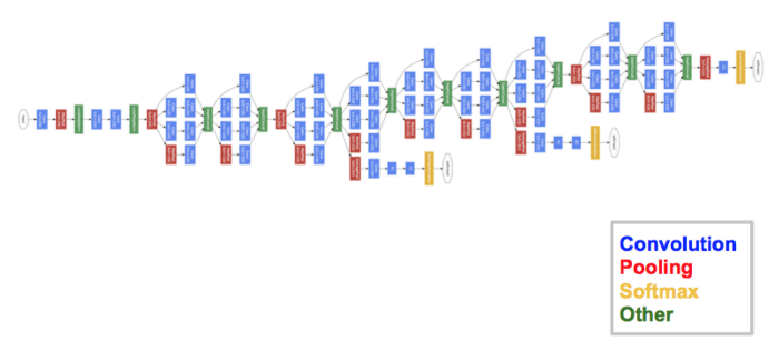
ILSVRC 2014 대회의 우승자는 Google의 GoogLeNet(Inception V1이라고도 함)이다. 6.67%의 상위 5위 오류율을 달성. 인간 수준의 성과에 매우 가까웠다고 한다. 27개의 pooling layer가 포함된 22개의 layer로 구성된다.
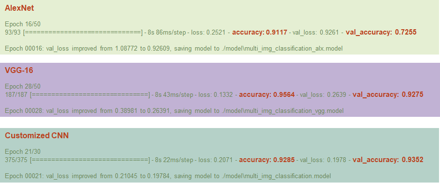
EarlyStopping을 했을 때 이미지 사이즈에 맞게 변형해서 만든 저희 모델들의 결과
VGG-16
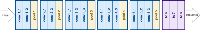
ILSVRC 2014 대회의 준우승은 커뮤니티에서 VGGNet이다. VGGNet은 16개의 컨볼루션 레이어로 구성되며 매우 균일한 아키텍처로 구성됐다. AlexNet과 유사한 3x3 회선만 있지만 필터가 더 많다. 이미지에서 특징을 추출하기 위해 커뮤니티에서 선호되고 있다. 단점은 훈련에 많은 시간이 걸리고, 네트워크 아키텍처 가중치가 크다.
이미지 크기 244x244
|
1
2
3
4
5
6
7
8
9
10
11
12
13
14
15
16
17
18
19
20
21
22
23
24
25
26
27
28
29
30
31
32
33
34
35
36
37
38
39
40
41
42
43
|
def vgg_16():
inputs = Input(shape=(64, 64, 3))
conv1_1 = Conv2D(filters=32, kernel_size=(3, 3), strides=1, padding="same", activation='relu')(inputs)
conv1_2 = Conv2D(filters=32, kernel_size=(3, 3), strides=1, padding="same", activation='relu')(conv1_1)
pool1 = MaxPooling2D(pool_size=(2, 2), strides=2, padding="valid")(conv1_2)
nor1 = BatchNormalization()(pool1)
conv2_1 = Conv2D(filters=64, kernel_size=(3, 3), strides=1, padding="same", activation='relu')(nor1)
conv2_2 = Conv2D(filters=64, kernel_size=(3, 3), strides=1, padding="same", activation='relu')(conv2_1)
pool2 = MaxPooling2D(pool_size=(2, 2), strides=2, padding="valid")(conv2_2) # 16
nor2 = BatchNormalization()(pool2)
conv3_1 = Conv2D(filters=128, kernel_size=(3, 3), strides=1, padding="same", activation='relu')(nor2)
conv3_2 = Conv2D(filters=128, kernel_size=(3, 3), strides=1, padding="same", activation='relu')(conv3_1)
conv3_3 = Conv2D(filters=128, kernel_size=(3, 3), strides=1, padding="same", activation='relu')(conv3_2)
pool3 = MaxPooling2D(pool_size=(2, 2), strides=2, padding="valid")(conv3_3)
nor3 = BatchNormalization()(pool3)
# 4 layers
conv4_1 = Conv2D(filters=128, kernel_size=(3, 3), strides=1, padding="same", activation='relu')(nor3)
conv4_2 = Conv2D(filters=128, kernel_size=(3, 3), strides=1, padding="same", activation='relu')(conv4_1)
conv4_3 = Conv2D(filters=128, kernel_size=(3, 3), strides=1, padding="same", activation='relu')(conv4_2)
pool4 = MaxPooling2D(pool_size=(2, 2), strides=2, padding="valid")(conv4_3) # 4
nor4 = BatchNormalization()(pool4)
# 5 layers
conv5_1 = Conv2D(filters=128, kernel_size=(3, 3), strides=1, padding="same", activation='relu')(nor4)
conv5_2 = Conv2D(filters=128, kernel_size=(3, 3), strides=1, padding="same", activation='relu')(conv5_1)
conv5_3 = Conv2D(filters=128, kernel_size=(3, 3), strides=1, padding="same", activation='relu')(conv5_2)
pool5 = MaxPooling2D(pool_size=(2, 2), strides=2, padding="valid")(conv5_3)
nor5 = BatchNormalization()(pool5)
drop5 = Dropout(0.5)(nor5)
flatten1 = Flatten()(drop5)
dense1 = Dense(units=2048, activation=tf.nn.relu)(flatten1)
dense2 = Dense(units=1024, activation=tf.nn.relu)(dense1)
logits = Dense(units=20, activation='softmax')(dense2)
return Model(inputs=inputs, outputs=logits)
model=vgg_16()
model.compile(loss='categorical_crossentropy', optimizer=otm, metrics=["accuracy"])
model.summary()
|
cs |
모델 성능 평가
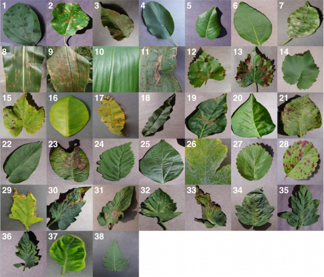
외부 데이터를 수집하려고 직접 찾아보면서 고생을 하다가, 관련 자료를 깃허브에 친절하게 올려주신 분이 있어서 감사히 썼습니다.
https://github.com/spMohanty/PlantVillage-Dataset/tree/master/raw/color
GitHub - spMohanty/PlantVillage-Dataset: Dataset of diseased plant leaf images and corresponding labels
Dataset of diseased plant leaf images and corresponding labels - GitHub - spMohanty/PlantVillage-Dataset: Dataset of diseased plant leaf images and corresponding labels
github.com
|
1
2
3
4
5
6
7
8
9
10
11
12
13
14
15
16
17
18
19
20
21
22
23
24
25
26
27
28
29
30
31
32
33
34
35
36
37
38
39
40
41
42
43
44
45
46
47
48
49
50
51
52
53
54
55
56
57
58
59
60
61
62
63
64
65
66
67
68
69
70
71
72
73
74
75
76
77
78
79
80
81
82
83
84
85
86
87
88
89
90
91
92
93
94
95
96
97
98
99
100
101
102
103
104
105
106
107
108
|
##########################
# 테스트 데이터 50개 랜덤으로 평가
##########################
########################################
#class name으로 변경
from os import rename, listdir
path2 = "./tests" #TEST_DATA => tests로 수정함
list3 = list(str(i) for i in range(20))
dict3 = dict(zip(combined_labels,list3))
for fname in os.listdir(path2):
newname = dict3.get(fname)
try:
if newname not in os.listdir(path2) :
os.rename(os.path.join(path2, fname), os.path.join(path2,newname))
except:
counter = True
if counter :
print("이미 변경 완료")
else :
print("class name으로 변경완료")
########################################
### 필수 아님 #####
#labeled_name으로 되돌리고 싶을 때
list3 = list(str(i) for i in range(20))
dict3 = dict(zip(list3, combined_labels))
for fname in os.listdir(path2):
newname = dict3.get(fname)
try :
if newname not in os.listdir(path2) :
os.rename(os.path.join(path2, fname), os.path.join(path2,newname))
except:
counter = True
if counter :
print("이미 변경 완료")
else :
print("labeled name으로 변경완료")
########################################
import os, re, glob
import cv2
import numpy as np
from sklearn.model_selection import train_test_split
from tensorflow.keras.preprocessing.image import img_to_array
import random
# class에 따른 본래 label
t_list = list(str(i) for i in range(20))
t_dict = dict(zip(t_list, combined_labels))
########################################
#테스트 데이터 list
tests ='./tests'
tests_list = os.listdir(tests)
model = load_model('model1.h5') # 자신의 model load
def convert_image_to_array(image_dir):
try:
image = cv2.imread(image_dir)
if image is not None :
image = cv2.resize(image, dsize=(64,64))
return img_to_array(image)
else :
return np.array([])
except Exception as e:
print(f"Error : {e}")
return None
def predict_disease(image_path, num):
global count
image_array = convert_image_to_array(image_path)
np_image = np.array(image_array, dtype=np.float32) / 225.0
np_image = np.expand_dims(np_image,0)
result = model.predict_classes(np_image)
c = result.astype(str)[0]
if c == num :
count += 1
return count
for i in range(20):
num = str(i)
tests_file = os.listdir(f'tests/{num}')
count = 0
max = len(tests_file)
for j in range(50):
ran_num = random.randint(0,max) # 임의의 숫자 추출
tests_path = f'tests/{num}/' + os.listdir(f'./tests/{num}')[ran_num]
predict_disease(tests_path, num)
print(f'###### 테스트 데이터 {t_dict.get(num)} 의 정확도 입니다 #######' )
print('accuracy: {:0.5f}'.format(count/50))
print('테스트 완료')
|
cs |
###### 테스트 데이터 Corn_(maize)_Common_rust_ 의 정확도 입니다 #######
accuracy: 1.00000
###### 테스트 데이터 Corn_(maize)_healthy 의 정확도 입니다 #######
accuracy: 1.00000
###### 테스트 데이터 Grape_Black_rot 의 정확도 입니다 #######
accuracy: 0.96000
###### 테스트 데이터 Grape_Esca_(Black_Measles) 의 정확도 입니다 #######
accuracy: 0.94000
###### 테스트 데이터 Grape_Leaf_blight_(lsariopsis_Leaf_Spot) 의 정확도 입니다 #######
accuracy: 0.98000
###### 테스트 데이터 Orange_Haunglongbing_(Citrus_greening) 의 정확도 입니다 #######
accuracy: 0.98000
###### 테스트 데이터 Pepper,_bell_Bacterial_spot 의 정확도 입니다 #######
accuracy: 0.94000
###### 테스트 데이터 Pepper,_bell_healthy 의 정확도 입니다 #######
accuracy: 0.98000
###### 테스트 데이터 Potato_Early_blight 의 정확도 입니다 #######
accuracy: 1.00000
###### 테스트 데이터 Potato_Late_blight 의 정확도 입니다 #######
accuracy: 0.98000
###### 테스트 데이터 Soybean_healthy 의 정확도 입니다 #######
accuracy: 0.96000
###### 테스트 데이터 Squash_Powdery_mildew 의 정확도 입니다 #######
accuracy: 0.94000
###### 테스트 데이터 Tomato_Bacterial_spot 의 정확도 입니다 #######
accuracy: 0.90000
###### 테스트 데이터 Tomato_Early_blight 의 정확도 입니다 #######
accuracy: 0.90000
###### 테스트 데이터 Tomato_Late_blight 의 정확도 입니다 #######
accuracy: 0.84000
###### 테스트 데이터 Tomato_Septoria_leaf_spot 의 정확도 입니다 #######
accuracy: 0.96000
###### 테스트 데이터 Tomato_Spider_mites_Two-spotted_spider_mite 의 정확도 입니다 #######
accuracy: 0.96000
###### 테스트 데이터 Tomato_Target_Spot 의 정확도 입니다 #######
accuracy: 0.96000
###### 테스트 데이터 Tomato_Tomato_Yellow_Leaf_Curl_Virus 의 정확도 입니다 #######
accuracy: 0.98000
###### 테스트 데이터 Tomato_healthy 의 정확도 입니다 #######
accuracy: 0.98000
테스트 완료
----------------------------------------------------------------------------------------------------
테스트 정확도 : 0.957

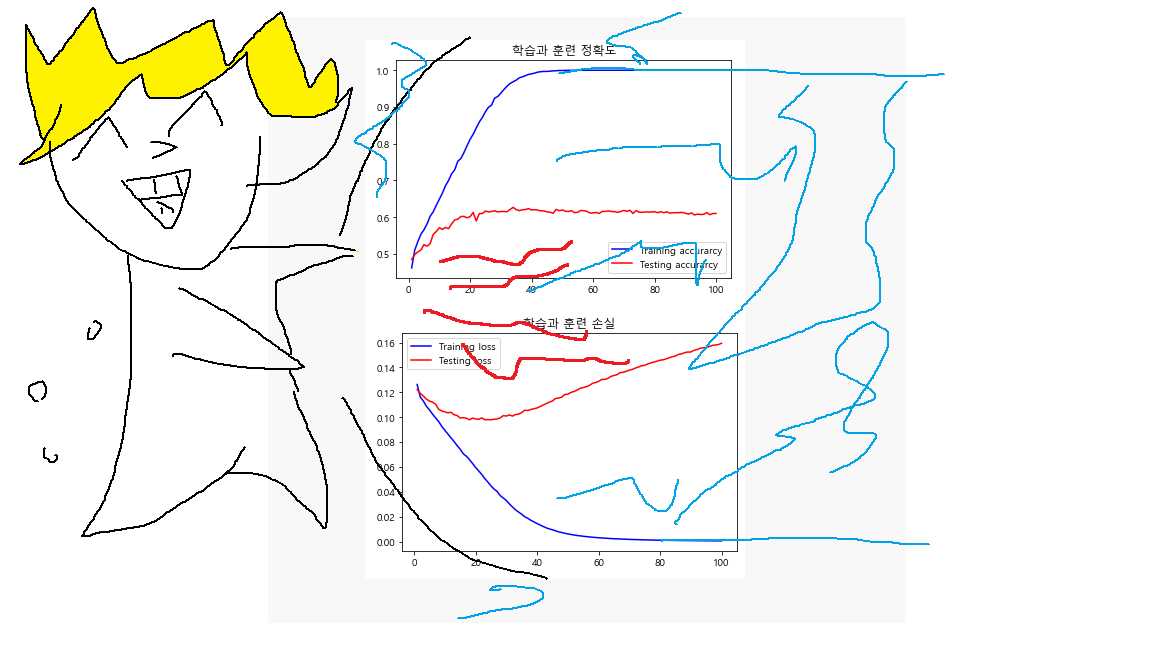
이건 팀원이 정확도와 loss 값 그래프를 보고 그린 그래프
수고하셨습니다
'도전하자. 프로젝트' 카테고리의 다른 글
| 4-2 파이썬 팀프로젝트 CNN 카테고리 분류 - 데이터 크롤링 및 전처리 (0) | 2021.08.10 |
|---|---|
| 4-1 파이썬 팀프로젝트 CNN 상품 카테고리 분류 intro (셀리니움 vs BS4) (0) | 2021.08.10 |
| 3-3 파이썬 프로젝트 CNN 식물 병충해 시각화 및 모델 개선 (0) | 2021.08.04 |
| 3-2 파이썬 팀프로젝트 CNN 모델링 - 인공지능, 머신러닝, 딥러닝 뭔데? (0) | 2021.08.01 |
| 3-1 파이썬 팀프로젝트 CNN 식물 병충해 분류 (0) | 2021.07.31 |